Introduction to NumPy

• Why do we need NumPy?
• NumPy overview
• The NumPy array
  • Creation
  • Save and load
  • Manipulation
  • Indexing
  • Copy vs view
• NumPy modules

Why do we need NumPy?

Python basic types

• Numbers: 10, 10.0, 1.0e+01, (10.0+3j)
• Strings: "Hello world"
• Bytes: b"Hello world"
• Lists: ["abc", 3, "x"]
• Tuples: ("abc", 3, "x")
• Dictionnaries: {"key1": "abc", "key2": 3, "key3": "x"}

Python basic operators

• +: Addition
• -: Substraction
• /: Division
• **: Exponentiation
• abs(x): Absolute value of x
• x % y: Remainder of x divided by y
• x // y: Quotient of the x divided by y

Operations on basic Python types

# Let a be a list
a = [1, 2, 3]
print(a)

# What is the results of
2 * a[2]

# and
2 * a
# is [2, 4, 6] the expected result?

# You can try other combinations of operations and data types.

Without additional libraries Python is almost useless for scientific computing.

Scientist's Swiss Army knife

• Numpy provides support for large, multi-dimensional arrays and matrices.
• Matplotlib provides support for high quality visualizations.
• SciPy provides additional scientific capabilities.

NumPy overview

NumPy is the library providing number crunching capabilities to Python, and enhances Python with tools for:

• treatment of multi-dimensional data
• access to optimized linear algebra libraries
• encapsulation of C and Fortran code

import numpy as np

The NumPy array

The np.ndarray object is:

• a collection of elements of the same type
• multidimensional with flexible indexing
• handled as any other Python object
• implemented in memory as a true table optimized for performance

It can be interfaced with other languages.

Array creation

# Create an array from a list of values.
a = np.array([1, 2, 3, 5, 7, 11, 13, 17])
a

# Create an array from a list of values and dimensions.
b = np.array([[1, 2, 3], [4, 5, 6]])
b

np.array?

Array creation with dedicated methods

Documentation: https://docs.scipy.org/doc/numpy/reference/routines.array-creation.html

np.empty((2, 4))

np.zeros((1, 3))

np.ones((2, 2, 3))

np.arange(start=0, stop=10, step=1)

np.linspace(start=0, stop=10, num=11)

np.identity(2)

Array access

a = np.array([1, 2, 3, 5, 7, 11, 13, 17])
# Access the first element
print(a[0])

# Access the second element
print(a[1])

b = np.array([[1, 2, 3], [4, 5, 6]])
# Access first-dimension elements (first row here).
print(b[0])

# Access the second element (column) of the first row.
print(b[0, 1])

Exercise

Use Python as a simple calculator and try the basic operations on Python lists and NumPy arrays.

a = [1, 2, 3]
b = np.array(a)

# Python list
print("2 * a[2] =", 2 * a[2])
print("2 * a =", 2 * a)

# NumPy array
print("2 * b[2] =", 2 * b[2])
print("2 * b =", 2 * b)

Types of elements

• Integers and real numbers with different precision
• Complex numbers
• Chains of characters
• Any Python object

The the element type can be specified using the dtype argument.

np.zeros((1, 3), dtype=int)

np.arange(3, dtype=np.float64)

a = dict({"key1": 0})
b = [1, 2, 3]
c = "element"
np.array([a, b, c], dtype=object)

https://numpy.org/doc/stable/reference/arrays.scalars.html#sized-aliases

• Integers: int32, int64, uint8 ...
• Real numbers: float32, float64 ...
• Complex: complex64, complex128

a = np.arange(10, dtype=np.float32)
print(f"The size of the array is {a.size * a.itemsize} bytes.")

a = np.arange(10, dtype=np.float64)
print(f"The size of the array is {a.size * a.itemsize} bytes.")

Structured/Record arrays

They allow access to the data using named fields. Imagine your data being a spreadsheet, the field names would be the column heading.

img = np.zeros((3,), dtype=[("r", np.float32), ("g", np.float64), ("b", np.int32)])
img

img["r"] = 1.0
img

Save and load

Documentation: https://docs.scipy.org/doc/numpy/reference/routines.io.html

a = np.arange(start=0, stop=10, step=1, dtype=np.int32)
a

# Save as a binary file (.npy).
np.save("data.npy", a)

np.load("data.npy")

# Save as a text file.
np.savetxt("myarray.txt", a, fmt="%d")

!cat myarray.txt

np.loadtxt("myarray.txt", dtype=np.int32)

Plotting NumPy arrays using Matplotlib

Matplotlib is a versatile plotting library that can be used to produce high-quality figures. It provides MATLAB-like functions, such as plot and imshow.

Integration in the notebooks can be enabled using %matplotlib magic.

%matplotlib inline
# %matplotlib widget (for interactive plots, but requires the ipympl package)
# %matplotlib nbagg

from matplotlib import pyplot as plt

x = np.array([0.0, 0.33, 0.66, 0.99, 1.32, 1.65, 1.98, 2.31, 2.64, 2.98, 3.31, 3.64, 3.97, 4.3, 4.63, 4.96, 5.29, 5.62, 5.95, 6.28])
y = np.array([ 1.0, 0.94, 0.79, 0.55, 0.24, -0.08, -0.4, -0.68, -0.88, -0.99, -0.99, -0.88, -0.68, -0.4, -0.08, 0.24, 0.55, 0.79, 0.95, 1.0])

fig = plt.figure()
plt.plot(y)
# plt.plot(x, y)

image = np.random.rand(100, 50)

plt.imshow(image)
plt.colorbar()

Exercise

Open the HPLC exercise notebook

Manipulation

Array operations

Common functions are:

• Linear algebra: matmul matrix multiplication, dot product, inner product, outer product
• Statistics: mean, std, median, percentile, ... (https://docs.scipy.org/doc/numpy/reference/routines.statistics.html)
• Sums: sum, cumsum, ...
• Math: cos, sin, log10, interp, ... (https://docs.scipy.org/doc/numpy/reference/routines.math.html)
• Indexing, logic functions, sorting
• See: https://docs.scipy.org/doc/numpy/reference/routines.html

a = np.linspace(0.0, 1.0, 100)
print("Mean:", np.mean(a), ", Standard deviation:", np.std(a))

# Standard operations operate element by element.
angles = np.linspace(0, np.pi, 5)
np.cos(angles)

a = np.array([[0.0, 1.0, 2.0], [3.0, 4.0, 5.0], [6.0, 7.0, 8.0]])
b = np.identity(3)
np.matmul(a, b) # Or equivalently a @ b

Array operations along an axis

Many NumPy reduction functions take an axis argument.

a = np.array([[0, 1, 2, 3], [4, 5, 6, 7]])
a

np.min(a)

np.min(a, axis=1)

Array methods

Some Numpy functions are also available as methods.

a = np.array([[7, 6, 5, 4], [3, 2, 1, 0]])
a

# Returns a value computed from the array
a.min(), a.max(), a.sum()

# An in-place sort operation.
a.sort(axis=1)
a

More on array methods

a = np.array([(0, 1), (2, 3)])
a

a.transpose()

np.transpose(a)

b = a.copy()
c = np.copy(a)
d = np.array(a, copy=True)

Be careful when using copy as it is shallow, and it will not copy object elements within arrays. For this, you need to use copy.deepcopy.

a = np.array([1, "m", [2, 3, 4]], dtype=object)
c = np.copy(a)
a[0] = 2
a[2][0] = -1
a, c

Array attributes

The dtype attribute identifies the type of the elements of the array.

a = np.array([[3, 2], [8, 12]])
a.dtype

a.dtype.name, a.dtype.str

The shape attribute is a tuple containing the array dimensions.

a = np.array([1, 2, 3, 4])
a.shape

# It can also be set.
a.shape = (2, 2)
a

More array attributes

• ndim: Number of dimensions
• size: Total number of elements
• itemsize: Size of a single item
• strides: Bytes to step in each dimension
• flags: Contiguity of the data in the buffer
• nbytes: Size in bytes occupied in memory
• data: Read/write buffer containing the data

a = np.array(
    [[1, 2], 
     [3, 4]])
a.ndim

Exercise

Continue the HPLC exercise notebook - Part II

Indexing

Select elements as with any other Python sequence.

• Indexing starts at 0 for each array dimension
• Indexes can be negative: x[-1] is the same as x[len(x) - 1]

a = np.array([0, 1, 2, 3])
print("a[0] =", a[0])
print("a[-1] =", a[-1])

a = np.array([(1, 2, 3, 4), (5, 6, 7, 8), (9, 10, 11, 12)])
a

a[2] # Select all the elements of the third row.

a[2, :] # Same as previous, assuming the array has at least two dimensions.

a[1, 2] # Select the element from the second row and third column.

a[0, -1]  # Select the last element of the first row.

a[0:2, 0:4:2]  # More elaborate indexing using the `start:stop:step` syntax.

More indexing

a = np.arange(10.0, 18.0)
a

# The index argument can be a list or an array.
a[[0, 3, 5]]

# The index argument can be a logical array.
mask = a > 13
print("a > 13 =", mask)
a[mask]

Assignment

a

a[0:2] = 5  # Assign new values to array elements.
a

Exercise

Continue the HPLC exercise notebook - Part III

Exercise

1. Calculate the element-wise difference between x and y?
2. Provide an expression to calculate the difference x[i+1]-x[i] for all the elements of the 1D array.

x = np.arange(10)
y = np.arange(1, 11)
print("x =", x)
print("y =", y)

# TODO

import exercicesolution

exercicesolution.show("ex3_1")

exercicesolution.show("ex3_2")

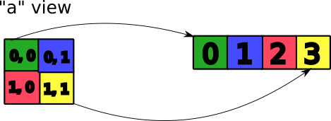
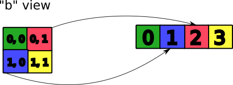
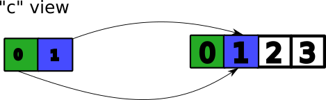
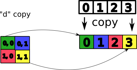
Copy vs view

You saw previously data copy. But you can work on the same raw data with different views (representations).

• copy: duplicate the data
• view: new array object pointing to the same data

a = np.array([[0, 1], [2, 3]])
b = a.transpose()
a, b

c = a[0]
c

d = a.copy()

a[0, 0] = 4

print("a:", a)
print("b:", b)
print("c:", c)
print("d:", d)

Exercise

Perform a 2x2 binning of an image

1. Binning with a 1D array

   • 1.1: Generate a 1D array with 100 elements in increasing order
   • 1.2: Perform a binning such that:

raw data: 1 2 3 4

binned data: 1+2 3+4

2. Binning with a 2D array 2x2 binning

   • 2.1: Generate a 100x100 2D array with elements in increasing order
   • 2.2: Perform a binning such that:

1	2	3	4
5	6	7	8
9	10	11	12
13	14	15	16

1+2+5+6	3+4+7+8
9+10+13+14	11+12+15+16

3. Set all elements of the resulting array that are below 1000 to 0.

# TODO

import exercicesolution

exercicesolution.show("ex4_1")

exercicesolution.show("ex4_2")

exercicesolution.show("ex4_2_alt")

NumPy modules

Documentation: https://docs.scipy.org/doc/numpy/reference

Linear algebra: numpy.linalg

• numpy.linalg.det(x): determinant of x
• numpy.linalg.eig(x): eigenvalues and eigenvectors of x
• numpy.linalg.inv(x): inverse matrix of x
• numpy.linalg.svd(x): singular value decomposition of x

np.linalg.det?

help(np.linalg.det)

Random sampling: numpy.random

Simple random data

# Random integers in the interval [low:high)
np.random.randint(low=0, high=5, size=10)

# Random floats in the interval [0.0:1.0)
np.random.random(10)

np.random.bytes(10)

Permutations

a = np.arange(1, 10)
a

# In-place element permutation
np.random.shuffle(a)
a

# Out-of-place permutation
np.random.permutation(a)

Statistical distributions

Normal (Gaussian), Poisson, etc.

data = np.random.normal(loc=1.0, scale=1.0, size=100000)

%matplotlib inline
from matplotlib import pyplot as plt

histo, bin_edges = np.histogram(data, bins=100)
bin_centers = (bin_edges[:-1] + bin_edges[1:]) / 2.
plt.plot(bin_centers, histo)
# Or: plt.hist(data, bins=100)

Fast Fourier Transform: numpy.fft

• numpy.fft.fft: 1D FFT
• numpy.fft.fft2: 2D FFT
• numpy.fft.fftn: nD FFT

Polynomials: numpy.polynomial

In NumPy, polynomials can be created, manipulated, and even fitted. Numpy provides Polynomial, Chebyshev, Legendre, Laguerre, Hermite and HermiteE series.

Exercise

• Write a function fill_array(height, width) to generate an array of dimensions (height, width) in which X[row, column] = cos(row) * sin(column)
• Time-it for height=1000, width=1000

Bonus: Do the same for X[row, column] = cos(row) + sin(column)

def fill_array(height, width):
    a = np

%timeit fill_array(1000, 1000)

# inefficient fill
import exercicesolution
exercicesolution.show("ex5_inefficient_fill")
%timeit exercicesolution.ex5_inefficient_fill(1000, 1000)

# naive fill
exercicesolution.show("ex5_naive_fill")
%timeit exercicesolution.ex5_naive_fill(1000, 1000)

# clever fill
exercicesolution.show("ex5_clever_fill")
%timeit exercicesolution.ex5_clever_fill(1000, 1000)

# practical fill
exercicesolution.show("ex5_practical_fill")
%timeit exercicesolution.ex5_practical_fill(1000, 1000)

# optimized fill
exercicesolution.show("ex5_optimized_fill")
%timeit exercicesolution.ex5_optimized_fill(1000, 1000)

# atleast_2d fill
exercicesolution.show("ex5_atleast_2d_fill")
%timeit exercicesolution.ex5_atleast_2d_fill(1000, 1000)

Speed is a question of algorithm. It is not just a question of language.

Implementation	Duration (seconds)
ex5_inefficient_fill	5.052937
ex5_naive_fill	0.886003
ex5_clever_fill	0.016836
ex5_practical_fill	0.014959
ex5_optimized_fill	0.004497
ex5_atleast_2d_fill	0.005262

Done on Intel(R) Xeon(R) CPU E5-1650 @ 3.50GHz

numpy v2

numpy version 2 is about to be released.

See migration guide

Additional resources

• Complete reference material: http://docs.scipy.org/doc/numpy/reference
• NumPy user guide: https://docs.scipy.org/doc/numpy/user
• Many recipes for different purposes: https://scipy-cookbook.readthedocs.io
• Active mailing list where you can ask your questions: numpy-discussion@scipy.org
• Internal data-analysis mailing list: data-analysis@esrf.fr

More exercises for the braves

Thanks to Nicolas Rougier: https://github.com/rougier/numpy-100:

• Create a 5x5 matrix with values 1,2,3,4 just below the diagonal.
• Create a 8x8 matrix and fill it with a checkerboard pattern.
• Normalize a 5x5 random matrix.
• Create a 5x5 matrix with row values ranging from 0 to 4.
• Consider a random 10x2 matrix representing cartesian coordinates, convert them to polar coordinates.
• Create random vector of size 10 and replace the maximum value by 0.
• Consider a random vector with shape (100,2) representing coordinates, find point by point distances.
• Generate a generic 2D Gaussian-like array.
• Subtract the mean of each row of a matrix.
• How to I sort an array by the nth column?
• Find the nearest value from a given value in an array.